A Class Divided: The 1970’s Class that Experienceed Simulated Discrimination in Prejudice and Privilege
A Class Divided:Public School Kids Experience Simulated Lesson in Segregation and Privilege
Teacher’s Note
A Class Divided is an encore presentation of the classic documentary on third-grade teacher Jane Elliott’s “blue eyes/brown eyes” exercise, originally conducted in the days following the assassination of Rev. Martin Luther King Jr. in 1968. This guide is designed to help you use the film to engage students in reflection and dialogue about the historical role of racism in the United States, as well as the role of prejudice and stereotyping in students’ lives today.
Because the film deals with racism and prejudice, it may raise deep emotions for both you. Some students may be confronted with privilege for the first time while others may see an affirmation of a lifetime of discrimination. As you see in the film, frustration, anger, and pain are not uncommon responses to being confronted with bias and inequity.
Issue Definition and Topic Background
Racism
Some people argue that racism is primarily a belief or attitude and that anyone who unfairly judges another based on race is racist. Others argue that racism is about action and systemic discrimination, so only those with the power to act, and not those who are the targets of discrimination, can be racist. Which argument do you find convincing and why? Is there a difference between racism and prejudice? If so, what is the difference?
Consider the following definitions. What are the differences between them? How do they compare with the dictionary definition of “racism”? How might some people benefit and others be hurt from the use of one definition over another?
“Racism couples the false assumption that race determines psychological and cultural traits with the belief that one race is superior to another.” –A World of Difference project of the Anti-Defamation League of B’nai Brith
“Racism is any attitude, action, or institutional structure which subordinates a person or group because of skin color.” –U.S. Commission on Civil Rights, 1970
“We define racism as an institutionalized system of economic, political, social, and cultural relations that ensures that one racial group has and maintains power and privilege over all others in all aspects of life. Individual participation in racism occurs when the objective outcome of behavior reinforces these relations, regardless of the subjective intent.” –Carol Brunson Phillips and Louise Derman-Sparks in Teaching/Learning Anti-Racism: A Developmental Approach, (Teachers College Press, 1997)
Privilege
One of the goals of the civil rights movement was to ensure equal opportunity for every U.S. citizen, irrespective of race. When the civil rights movement began, the legal system did not grant the same rights to blacks and other minorities as it did to whites. Today, those laws have been changed, leading some to argue that the U.S. has achieved a level playing field for all. Is the field level? Is success based exclusively on merit and luck, or is race-based “privilege” still a factor? How was affirmative action policy crafted to address issues of privilege? Has it been successful?
Consider the following definitions. What are the differences between them? How do they compare with the dictionary definition of “privilege”?
· “unearned power conferred systemically” (Source: Peggy McIntosh, 1995)
· white privilege (hwait ‘privilidz), social relation, [ad. L. privilegi-um a bill or law in favor of or against an individual.] 1. a. A right, advantage, or immunity granted to or enjoyed by the class of white persons beyond the common advantage of all others; an exemption in many particular cases from certain burdens or liabilities. b. In extended sense: A special advantage or benefit of white persons; with ideological reference to divine dispensations, natural advantages, gifts of fortune, genetic endowments, social relations, etc. 2. A privileged position; the possession of an advantage white persons enjoy over non-whites and white individuals enjoy over non-white individuals. 3. a. The special right or immunity attaching to white persons as a social relation; prerogative. b. display of white privilege, a social expression of a white person or persons demanding to be treated as a member or members of the socially privileged class. (Source: The Monkeyfist Collective (Links to an external site.))
Thinking About It
Essential questions will guide your thinking. Questions and statements are designed to you to process the information from the documentary. These are not the prompt. You do not need to directly answer these questions. Use them to organize your thoughts and focus your attention toward key details to use in referencing examples and evidence to support your critical response.
· How do our beliefs about our response towards expectations of our government’s political response to social practices influencing the ways in we see and choose to interact with each other?
· What happens when one aspect of our identities is used to sort us into groups?
· How has our response to difference and what we do with a variation influence politics and American government?
· How does the aspect in our self identity cause collective political effects on society’s expectation of government’s role?
· How does our identity affect how we see not only ourselves, how how see others, and the choices that we ultimately make.
· What is the relationship between self determining identification and political preferences towards government decisions and actions
Teacher’s Note
Change your thinking to learn a broadened understanding of political perspective. There are always two interpretations of a word’s single definition. Webster’s sets a common standard with word definitions that make understanding more general and less exclusive. Diversity is a uniqueness that requires awareness of personal exclusivity. Limited understanding comes from limited perspective. A word that is clearly defined, is the most accepted word. Self imposed limitations that have failed us to know both sides of a words meaning.
A word’s definition needs to be seen for both what it IS and what it IS NOT. Apply the both sides of a definition specifically to the words “decisions and actions” mentioned in the previous section.
Decisions and actions need to be defined with relation to what IS NOT if we want to broaden our perspective self identify politics that shape government response….AND most importantly shape their non-response.
Learning Materials
Watch the entire movie in order to respond to the prompt
Prompts
Select one of the following prompts to write your reflective writing paper on
1. What does Elliott’s classroom experiment suggest about what can happen when one aspect of our identities is valued more than all of the others?
2. While eye color may not be related to power in our society, what are aspects of identity that give some people more power and privileges than others? Who determines which differences matter? Why do individuals and groups either go along or not go along with these decisions?
3. How do beliefs about differences in our society shape the way we see ourselves and others? How do they shape the way others see us? How do beliefs about differences in our society shape the way we respond when we encounter an individual or group that is different from us?
Hydrographics are applied to firearms for aesthetic purposes almost as often as they are for functional ones. This is evident in the many different films available which are purely for looks. Let’s face it, you are unlikely to ever be surrounded by flames and skulls and in need of a firearm which blends into your environment. Consider all the purely aesthetic hydrographics you have seen and then discuss the following.
Do you find there to be any ethical concern with taking a tool such as a firearm and giving it a “designer look” like you would a car, boat, or other “toy”? Why or why not? If you were to offer hydrographic application at your own shop, would you apply these finishes if a customer requested them? Why or why not? Finally, how would you defend your position to a customer who took offense to your view, whatever it is?
1. A manufacturing facility that makes steel materials handling devices such as hand carts and an assortment of roller carts for moving heavy materials around in manufacturing facilities has decided to start making cantilever storage racking systems. This will require the purchase and installation of a 12-foot hydraulic press brake and a 12-foot shear in the fabrication department along with the necessary tools and dies to bend and punch holes in the rack components that will largely be manufactured from formed sheet metal. Employees have experience working smaller versions of this type of equipment, but room will need to be made and larger pieces of sheet metal will need to be cut and handled. The department will also need to continue to produce existing orders while the new equipment is installed. How can a management of change program be used to reduce risks in such a scenario? (75 words)
2. Your organization, a company that manufactures fitness equipment such as treadmills and elliptical machines, is about to introduce lean concepts into its operations in order to be more competitive with foreign manufacturers. The foreman from the assembly department, however, does not think that his employees have the time to be involved with the lean initiative. Provide a convincing argument about why it is important for the assembly line workers to play a part. (75 words)
3. Your purchasing department does not want to buy adjustable hydraulic pallet stands for the filter assembly line at a company that makes oil filters for cars and trucks. They state that the current process works just fine and that expensive, adjustable stands are not required in the Occupational Health and Safety Administration standards. The production employees in the facility are largely female and many have worked at the facility for decades. The current process for accessing filter parts entails having assemblers bend over to pick up arm loads of the various filter components from a pallet or bin and placing them on a table beside their respective workstations. The parts are assembled and pressed into place, and the completed product placed in a separate bin. Please provide a risk-based argument as to why the adjustable pallet stands would be the better choice. (200 words)
A manufacturing facility that makes steel materials handling devices such as hand carts and an assortment of roller carts for moving heavy materials around in manufacturing facilities has decided to start making cantilever storage racking systems
You were recently hired as the fleet safety manager for a small distribution company in the Midwest. Your small company just received a compliance, safety, and accountability (CSA) score of 81. Last month, your score was 77. Upper management has requested a review of the scores and your analysis of the company’s fleet safety performance.
Is that a good or bad score? Is a higher score better (like basketball), or is a lower score better (like golf)?
If it is a good score, what will you do to sustain your success?
If it is a bad score, describe what you are going to do to improve your score and to avoid having your fleet shutdown.
Recommend benchmarking and record-keeping systems for the company.
Identify performance incentives that you think would benefit the company’s fleet safety
Q1. You take a soil sample from your field, weigh it moist, oven-dry it, and weigh it dry. If the initial weight is 77 g and the final weight is 62 g, what is the gravimetric water content? If you know from previous soil sampling that the bulk density is 1.25 g cm-3, what is the volumetric water content? Make sure to show your work for full credit!
Q2. How much monoammonium phosphate (MAP) would you need to apply to an onion crop to get 30 lbs. N per acre if the fertilizer bag reads 11-52-0? How much phosphorus and potassium would this supply in oxide forms?
The Federal Housing Finance Agency (FHFA) was established by the Federal Housing and Reform Act of 2007 in order to regulate several government sponsored entities (GSE’s), particularly Fannie Mae, Freddie Mac and the Federal Home Loan Bank (FHLB)
Please pick one GSE and discuss with the class how your choice impacts real estate finance. Please follow the underwriting standards, underwriting tools, and overall organization. 250 words or more.
Please Use Headlines
The headlines I would expect would be:
Government entity
Under this headline, I would briefly (but more than one sentence) state the entity you are going to discuss. Give a little background of the entity to show you understand what it does.
I would then look back at the question and use the following three headlines (taken from the line, “Pay particular attention to their underwriting standards, underwriting tools, and overall organization.”
Underwriting Standards
Under this headline, I would discuss the underwriting standards of that agency.
Underwriting Tools
Under this headline, I would discuss the underwriting tools of that agency.
Overall Organization
Under this headline, I would discuss the overall organization of that agency.
A galaxy is an assembly of between a billion (109) and a hundred billion (1011) stars. In addition to stars, there is often a large amount of dust and gas, all held together by gravity. The Sun and the Earth are in the Milky Way Galaxy (sometimes referred to as “the Galaxy”). Galaxies have many different characteristics, but the easiest way to classify them is by their shape (or “morphology”), and Edwin Hubble devised a basic method for classifying them in this way. In his classification scheme, there are three types of galaxies: spirals, ellipticals, and irregulars.
Spiral galaxies were the first to be discovered, because the most luminous galaxies close to the Milky Way are spirals. These galaxies get their name from the spiral distribution of light seen in photographs. A subclass of spirals contains the barred spirals. Ordinary spirals have a nucleus which is approximately spherical, while barred spirals have an elongated nucleus which looks like a bar. Spirals are labeled as Sa, Sb, or Sc; barred spirals are designated SBa, SBb, or SBc. The subclassification (a, b, or c) refers both to the size of the nucleus and the tightness of the spiral arms.
Elliptical galaxies are classified according to the relative sizes of their apparent major and minor axes. All elliptical galaxies have n between 0 and 7.
Irregular galaxies have no obvious spiral or elliptical structure. It is thought that many irregulars were once spiral or elliptical, but that a close encounter with a larger galaxy disrupted the organization of the material by gravitational forces. Irregular galaxies come in two flavors: Irr I’s are resolvable into individual stars, and Irr II’s are not.
Not all galaxies are easily classified. Quasars are the bright, superluminal cores of very distant active galaxies. These galaxies are so distant in fact that the quasars look like stars in most images. However, their redshifts are so high that we know that they can not be stars. These quasars are moving away from us at extremely high velocities. Quasar 3C273, for example, is moving away from us at 43,700 km/sec!
The relationship between galaxy types is not clear. Because there is little evidence of star formation in elliptical galaxies, and because they seem to have extremely small angular momentum, it was thought that perhaps elliptical galaxies are much older than spirals. If this is true, then we would expect to see more spiral galaxies as we look farther out into the universe (that is, back in time). Recent observations made by Hubble Space Telescope do show more spirals in distant clusters of galaxies, however, there are also many more distorted galaxies and blue irregulars with enormous star formation rates.
We do know that there is a correlation between the environment and the type of galaxy that formed there. Dense clusters have much higher percentages of elliptical galaxies, indicating that dense galaxy formation regions are more likely to form ellipticals. The entire problem is not yet well understood, and many explanations rely heavily on the postulated existence of dark matter.
In the late 1920’s, Edwin Hubble discovered one of the most fundamental properties of the universe, namely that it is expanding in all directions with a speed proportional to the distance. He used the redshift of spectral lines from distant galaxies (calculated by Slipher) whose distances could be determined by other means (for example, by Cepheid variable observations or measuring the angular sizes of HII regions). He interpreted the observed spectral shift as a Doppler shift, and determined that all galaxies (except a few very close ones that are in the same group of galaxies as the Milky Way) are receding from the Milky Way Galaxy with speeds proportional to their distances:
v=H·d,
where d is the galaxy’s distance (in Mpc), H is Hubble’s constant (with a modern value of about 65 km/s/Mpc), and the speed v is found from the Doppler shift of the galaxy.
Procedure
Galaxy images, click each.
1. NGC 1381 2. NGC 1398 3. NGC 224 4. NGC 3031 5. NGC 3384 6. NGC 5055 7. NGC 5184 8. NGC 5236 9. NGC 7331 10. 3C273
1. Examine the images of the galaxies listed above. When there is more than one galaxy in the
image, use the finder chart to identify the galaxy in question. 2. Fill in the table (this is worth 10 pts)
3. Identify each galaxy’s type. 4. Estimate the subgroup of the spirals using this image. 5. For ellipticals, measure the major and minor axes of the ellipticals
a. You can calculate the subclass. Use any scale (inches or millimeters) you like to measure the major and minor axes, but be sure to measure both axes on the same scale.
b. For example, the longest dimension becomes the A value. Measure it in centimeters or inches. Measure the dimension perpendicular to that one as the B value.
c. Calculate the n value by dividing a by b. So, an E2 is an elliptical galaxy that is 2x as long as it is wide.
d. Note: you only need to measure the axes for the elliptical galaxies! 6. Use the Hubble constant and the formula given in the “Background and Theory” section
above to find the distance to each galaxy. a. Remember the assumptions behind Hubble’s Law. b. Convert the distance from Mpc to light years. (1 Mpc = 3.26·106 l.y.) c. Converting to light years gives the amount of time the light traveled between leaving
the galaxy and arriving at the telescope. d. Check to make sure that all of your answers make sense. e. For example, check that none of the galaxies’ light has been traveling for more than the
age of the Universe. 7. It is often difficult to make astronomical numbers meaningful.
a. For each of the galaxies, indicate what was happening in the Earth’s history when the light left that galaxy.
b. For example, the dinosaurs became extinct about 65 million years ago, Pangaea split into multiple continents about 200 million years ago, the Earth is about 4.5 billion years old, and the Universe is about 15 billion years old. Find these dates using the cosmic calendar in Chapter 01 or elsewhere on the Net.
Part 1 Questions (3 pts each)
1. What color do these galaxies tend to be (some areas may be saturated and look white, so look closer to the edge)? If different regions are different colors note that.
2. The velocity of NGC224 is negative. What does this mean? What are the implications for applying the Hubble Law to this galaxy?
3. 3C273 is one of the brightest radio sources in the sky. But the type of galaxy 3C273 is impossible to find from these images. Does this make sense? Hint: Look at the distance.
Galaxies — those vast collections of stars that populate our universe — are all over the place. But how many galaxies are there in the universe? Counting them seems like an impossible task. Sheer numbers is one problem — once the count gets into the billions, it takes a while to do the addition. Another problem is the limitation of our instruments. To get the best view, a telescope needs to have a large aperture (the diameter of the main mirror or lens) and be located above the atmosphere to avoid distortion from Earth’s air. Perhaps the most resonant example of this fact is the Hubble eXtreme Deep Field (XDF), an image made by combining 10 years of photographs from the Hubble Space Telescope. The telescope watched a small patch of sky in repeat visits for a total of 50 days, according to NASA. If you held your thumb at arm’s length to cover the moon, the XDF area would be about the size of the head of a pin. By collecting faint light over many hours of observation, the XDF revealed thousands of galaxies, both nearby and very distant, making it the deepest image of the universe ever taken at that time. So if that single small spot contains thousands, imagine how many more galaxies could be found in other spots.
Procedure
1. Look at this Hubble Ultra Deep Field (UDF) image segment. Note there are no stars, only galaxies in this image. Light from most of the galaxies in this image left when the universe was about 1 billion years old, so they provide the earliest snapshot yet of what galaxies were like when the universe was young.
2. Take the portion of sky imaged by the telescope and count the number of galaxies a. In this case, you can either print out the image and take a ruler to one corner and make
a square and count the number of galaxies in that square. b. OR you could not print it out and instead do the same thing on your monitor – just use
two pieces of paper, taped carefully to the edge of the monitor to make a paper square outline. Count the number of galaxies inside that square.
3. Then — using the ratio of the square to the entire image — you can estimate the number of galaxies in the whole image.
a. Measure the whole image using a ruler, both sides. b. Multiply the two sides to get the area of the whole image. c. Now measure the two sides of your measured square. d. Make the scaling factor – area of whole image divided by area of measured square. e. Estimate the total number of galaxies by multiply your value from 3d above by the
number of galaxies you actually counted (answer 2a or 2b above).
Questions (4 pts each)
1. Estimate the number of galaxies in the image. Describe how you estimated the number. 2. Estimate the number of galaxies you can classify as spiral, elliptical or lenticular. What fraction
of the total number of galaxies is this? 3. Estimate the number of irregular galaxies. What fraction of the total number of galaxies is this? 4. How is the Hubble classification system useful for the galaxies in the UDF? What does this
Each person in a group should contribute equally to get the same grade. You have to mention the Percentage contribution of each person in your Project report.
————————————————————————————
Rubrics /Grade breakdown:
Report (100pts)
Theory, Procedure, Data, Analysis, and conclusion
THEORY (10pts): Briefly explain the underlying physical principle and exactly what you want to test.
PROCEDURE (30pts): Explain what you did, at a level such that someone in your class could reasonably reproduce your results. Include at least one diagram.
DATA (20pts): Include data tables (can be LaTeX’d, word doc’d, excel’d, pictures of hand-drawn tables, etc – as long as they’re legible, we’re happy). Explain the meaning of any variable you introduce. Include uncertainties. (Note that having poor data and explaining what went wrong is much, much, much better than fudging your data. One is a reasonable thing to do, and the other is academic dishonesty.)
ANALYSIS (20pts): Explain how you got from your data to your result. No need to show every step of your derivations, but give enough explanation that a classmate could reproduce your results.
CONCLUSION (20pts): What did you find? Numbers should include uncertainties. What went wrong? What might have affected your results (sources of error)? How could the experiment be improved?
————————————————————————————————
——————————————————————————–
Abstract:
Force and motion is a universal concept that applies to all matter in the universe. Motion is the changing of position or location which requires a force to cause that change. Forces influence objects that are at rest or that are already in motion. In the three laws of motion proposed by Isaac Newton, it involves the notion of inertia, mass, velocity, and momentum. These laws and factors contribute to the driving force that helps apply the concept of force and motion that we experience everyday. Using the online simulation provided by the Phet website, we will be conducting experiments involving force and motion.
Introduction:
In lecture as well as additional readings from our textbook, we have been introduced to the different aspects and rules that apply to the world of physics. There are three important notions that Isaac Newton proposed when he first studied and introduced the motion of objects. He stated that (1) a stationary object will remain stationary unless an external force acts on it, (2) the change in an object’s motion is proportional to the force acting on it, and (3) every force has an equal and opposite force.
By using the online simulation, we aim to demonstrate the concept of force and motion with the provided resource. The simulation should be able to provide results that would mimic the experiment if we were to do it in person. The data and calculations taken from the experiment will be able to showcase the theory behind force and motion and give us a better understanding behind it. With both concepts, we will learn all the factors that play a part in force and motion and it will give us a deeper understanding behind what is needed to put something into motion as well as what type of force and how much force is needed to create that motion.
Theory:
With respect to Newton’s Second Law of Motion, we can understand the significance of the relation between force, mass, and acceleration. Under the circumstances of the experiment and in real life situations, force is simply a push or pull that acts upon an object. Furthermore, force is a vector quantity, in which it accounts for magnitude and direction. Newton’s Second Law regards the function of such objects for which all prevailing forces are not balanced.
As forces become unbalanced – another vector quantity – acceleration emerges. Acceleration directly depends on the net force which is the sum of all forces acting upon an object. As the net force increases, so does the acceleration. As the net forces decrease, so does the acceleration. On the other hand, acceleration inversely depends on an object’s mass in which the acceleration decreases as the mass increases. If the mass were to decrease, then acceleration would increase.
As Newton’s Second Law may be expressed verbally, it can also be explained mathematically. As force has direction we may find different forces along the experiment, the first equation will be used to find the net force:
FNet = F1 + F2 + F3+…
The second equation will be used to find the weight of such object:
Fw = mg
The magnitude of the weight is equivalent to the magnitude of the normal force, this can be expressed in the equation:
Fn = Fw
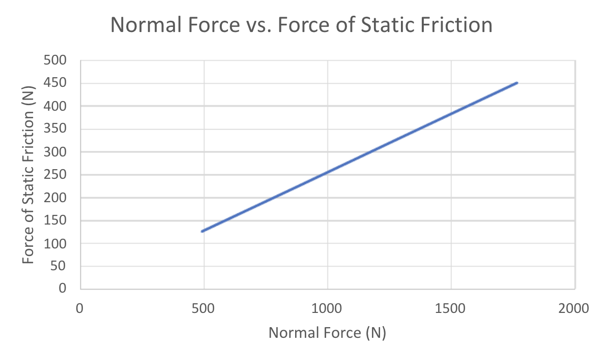
We will not only be calculating with equations but also graphs. We will be using google excel to make graphs and the slope in the graph will identify the coefficient of friction (μ). In the case of using the equation (shown below) we can find static and kinetic friction:
(Static Friction) Fs = μsN
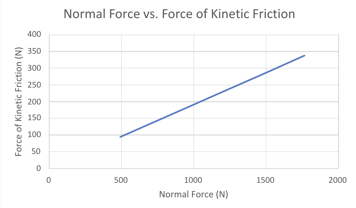
(Kinetic Friction) Fk = μkN
Experimental Apparatus & Setup:
Due to unfortunate circumstances of the COVID19 pandemic, our experimental setup was affected. Providentially, we were able to continue with the help and efforts of the Phet Colorado website. For this project, our experimental apparatus and setup consist of a virtual simulation from the website mentioned. This virtual simulation allows us to experiment and collect data that pertains to forces and motion, hence, the title of the project. In addition, we used our knowledge from this course, while applying “Chapter 4: Forces and Newton’s Laws of Motion” and “Chapter 5: Applications of Newton’s Laws.” The equipment needed to perform the experiment is all provided in the simulation.
Within the simulation setup, there are four selections to choose from:
The first selection is titled Net Force, in which the simulation consists of a “tug of war” between a number of figures. There are four blue figures and four red figures, with both colored teams having different sizes of figures. The number of figures that go on the left and right of the rope is adjustable, as it will eventually be the forces applied onto the object. The purpose of this simulation is to explain how objects will remain stationary unless external forces act on it.
The second selection is in regards to Motion, in which the figure model will be exerting force on an object that is mounted on a skateboard. The purpose of this simulation explains how the change in an object’s motion is proportional to the force acting on it with or without the application of mass(s) from the objects and figures provided.
The third selection focuses on friction. It’s similar to the Motion simulation, except that the crate isn’t mounted on the skateboard. Therefore, a friction force will affect the object in motion. The purpose of this simulation is to explain how an object’s motion is proportional to the force acting on it as well as how it can also come to terms with how every force has an equal and opposite force.
Finally, there’s an Acceleration simulation, where we can calculate the acceleration, based on the mass and friction that is applied on the crate. The figure model will push and launch the crate at a given amount of force, with and without applied mass on the crate, in which the acceleration will be given and calculated. The purpose of this simulation ties the whole notion of Newton’s Second Law of Motion together and explains the relationship between acceleration, mass, and all forces.
For all four selections of the simulations, we can insert various inputs to each simulation, such as a figure(s), a box, a trash bin, a gift box, a refrigerator, and a bucket of water, all providing different quantities in mass, speed, direction, and force.
Procedure:
Part 1
This part concludes Newton’s Second Law of Motion in which the concerning object will remain stationary unless external forces act on it. In this case, we add force to the right and left side of the cart to make it either move or remain stationary. We will find out how the forces affect the magnitude, the velocity, and the direction of the resultant force as well as the object (a cart).
Start the simulation by clicking on “Net Force”
Click on all the checkboxes on the upper righthand corner that indicate “Sum of Forces, Values, and Speed”
There are 8 stick figures located on the bottom; 4 blue figures and 4 red figures, drag the figures to the left and right side of the cart
After dragging the figures, make sure that the left rope has a force of 200N and the right rope has a force of 150N
Note the magnitude, direction of the resultant force and direction of where the car moved
Observe the velocity of the car, this can be found on the speedometer
Click on “Go” to start the simulation
Repeat steps 3-7, but this time, make sure that the left rope has a force of 200N and the right has a force of 200N
Part 2
This part concludes Newton’s Second Law of Motion in which the change in an object’s motion is proportional to the force acting on it. In this case, we are introducing mass and applying a force to the object (crate on skateboard) so it will start moving. We will find out how mass affects the motion of the object as it will cause it to either decelerate or accelerate.
Start the simulation by clicking on “Motion”
Click on the checkboxes located on the upper righthand corner that indicate “Forces, Values, Masses, and Speed”
There are objects with masses located on the bottom, drag such objects on top of the skateboard (we will be using a 50kg crate)
After dragging the object, set the “Applied Force” to 500N as it will start to push the crate on the skateboard
The simulation will start
Note the mass
Note the magnitude and the direction of the resultant force
Observe the velocity of the car, this can be found on the speedometer
Part 3
This part concludes Newton’s Second Law of Motion in which an object’s motion is proportional to the force acting on it. In this case, frictional force will be a part of the net forces. It can also come to terms with how every force has an equal and opposite force. In this case, friction force may be equal to the applied force. We will find out if frictional force is strong enough to either keep the object (a crate) at rest or moving.
Start the simulation by clicking on “Friction”
Click on the checkboxes located on the upper righthand corner that indicate “Forces, Sum of Forces, Values, Masses, and Speed”
There are objects with masses located on the bottom, drag such objects onto the simulation (we will be using a 50kg crate)
Apply force and increase it until it moves
Record the maximum force that keeps the object at rest
Record the force needed in order to make the box move
Note the masses, magnitude and direction of the forces and the resultant force
Part 4
This part concludes Newton’s Second Law of Motion in a similar way to all 3 parts above. We will be applying force and mass, as this experiment includes friction. We will find out how all these factors affect acceleration.
Start the simulation by clicking on “Acceleration”
Click on the checkboxes located on the upper righthand corner that indicate “Forces, Sum of Forces, Values, Masses, Speed, and Acceleration”
There are objects with masses located on the bottom, drag such objects onto the simulation (we will be using a 50kg crate)
Apply force and increase it until it moves
Record the maximum force that keeps the object at rest
Record the force needed in order to make the box move
Note the masses, magnitude and direction of the forces and the resultant force
Repeat steps 3-7, but add mass each time
Data:
One equation that is needed is one to find the resultant forces:
F = F1 + F2 + F3 . . .
Another equation used was one to find the weight:
Fw = mg
Another equation we used was to find the magnitude of the normal force:
Fn = Fw
To find the slope we used:
m = y2 – y1 / x2 – x1
The formula we used to find the forces of static and kinetic friction are:
Fs = ????sN and Fk = ????kN
This first table is the data of an object with certain mass values to start moving the object
Mass (kg)
Weight (N)
Normal Force (N)
Force of Static Friction (N)
50
491
491
126
90
883
883
226
130
1275
1275
326
150
1472
1472
376
180
1766
1766
451
This second table is the data of an object with certain mass values to keep the object moving
Mass (kg)
Weight (N)
Normal Force (N)
Force of Kinetic Friction (N)
50
491
491
94
90
883
883
169
130
1275
1275
244
150
1472
1472
281
180
1766
1766
338
Analysis: (Explain how we got the data)
Insert here
Conclusion:
In our lab experiment, there was definitely room for error. We used a website to conduct our experiment. Therefore, some of the things that may have gone wrong may occur due to technical, human, and instrumental error. An example of technical error would be how sometimes the object would move on its own without any force applied to it. A human error is not being able to read the results that we got or putting the right units. An instrumental source of error was that we could not see what speed our object was going. If this experiment was conducted in real life, an error would be how environmental factors such as the wind changes the direction or speed of the object.
In this experiment we explored the notions of Newton’s Second Law of Motion. The law formally states that acceleration occurs when a force acts on a mass and the greater amount of force on an object is needed when that mass of an object is greater. In our lab we conducted it into three parts; net force, motion, and friction. In terms of force, the experiment simply shows that if we move an object with force it will move. In terms of motion, the experiment explains with graphs, that if we put force over time the velocity would increase rapidly over the time. In terms of friction, the experiment illustrates in the graphs that friction increases when the object has motion; we can conclude that the opposing force is the friction force. Overall the results of the lab experiment exemplified the principles of Newton’s Second Law of Motion.
References
Phet Colorado simulation – Forces and Motion: Basics
Starting around 1972, Computed Tomography is consistently being created phenomenally, eminently with the assistance of software engineering, which has permitted making exceptionally exact diagnostics. CT advancement went through a few phases, from the model of Hounsfield to going through the consecutive and helical modalities. This advancement made CT a vital assessment in radiology (Kanne & Lin, 2018). In any case, this radiological strategy is the most lighting contrasted with different procedures; it can convey a portion of 50-500 times more prominent than a standard radiological assessment. Some patients can have life-altering effects after having a CT scan, but others oppose having the scan done, due to cancer risk. Studies have shown that the scan has a low risk of cancer-causing agents in the body (Pontone, G). To assess the danger to patients from CT checks, a gauge of the dose delivered to the skin and organs of a patient is fundamental. A need in this way exists to decide proper dosimetric amounts, for example, the organ dose and peak skin dose (PSD) (De las Heras).
The Federal Drug Administration (FDA) states that the Peak Skin Dose is the “highest radiation dose accruing actually at a single site on a patient’s skin.” Knowing the appropriate highest dosage is vital so that no harm is caused to the patient. The United States has regulated that the” fluoroscopic system provides a display of the irradiation time, dose rate at the interventional reference point during irradiation, and the cumulative dose for the procedure upon completion of irradiation” (Pontone, G). In preparation for actual patients, technologists and physicists would revert to the manufactured dose estimation which is called the Computed Tomography Dose Index (CTDI). The CTDI is generally utilized for quality control including the radiation output of CT machines. Specifically, the volume CTDI is shown on the control center of all CT machines and is promptly accessible to the administrator. In any case, the CT Dose Index (CTDIvol) was originally designed as an index of dose associated with various CT diagnostic procedures, not as a direct dosimetry method for individual patient dose assessments.
Moreover, CTDIvol is reported in two units: a 16-cm phantom for head exams or 32-cm phantom or body exams. The relationship between the CTDIvol and airiest dose depends on various factors, two of which are the patient size and composition. CTDIvol is displayed on the console of CT scanners, and it gives genuine estimates of the dose being delivered to patients and can serve to approve Monte Carlo recreations (Jones, A. Kyle). Specifically, estimating Peak Skin Dose is ideal since it is a surely known dosimetric amount that directly identifies with radiation-incited skin wounds. Besides, estimation estimates of PSD values, utilizing appropriate phantoms can without much of a stretch be made across all types of CT units and scan protocols accessible in clinics (Tack & Gevenois, 2018). This is significant for comparing doses for a similar CT examination in different facilities, which can change fundamentally. More recently, modifications to the original CTDI concept have attempted to convert it into to patient dosimetry method, but have mixed results in terms of accuracy.
Nonetheless, CTDI-based dosimetry is the current worldwide standard for estimation of patient dose in CT. Therefore, CTDIvol is often used to enable medical physicists to compare the dose output between different CT scanners. Also, since CTDIvol estimates the patient’s radiation exposure from the CT procedure, the exposures are the same regardless of patient size, but the size of the patients is a factor in the overall patient’s absorbed dose (SSDE). The size-specific dose estimate (SSDE) is measured in mGy, and it is a method of estimating CT radiation dose that takes a patient’s size into account.
From a radiation protection point of view, determining the maximum dose delivered to the skin would allow deriving quantities that can be compared with dose reference levels set by national and international standards. The most important outcome from a radiation safety perspective is evaluating if a radiation injury had occurred quickly (NCRP Report 116.) In this research, the peak skin dose delivered to a patient was estimated experimentally by measuring the dose delivered to the surface of the NEMA phantom and 32 cm CTDI phantom using external dosimeters. These dosimeters will provide PSD values for a given protocol and its related CTDIvol. From this, a relationship can be evaluated between both quantities. The aim of this project was to test the hypothesis that the size-specific dose estimate (SSDE) has a sufficiently strong linear relationship with PSD to allow direct calculation of the PSD directly from the SSDE.
Materials and Methods:
The measurements were performed with a Siemens 64 slices, Biograph mCT. A comparison was made between the CTDIvol value displayed on the CT console and the measured CTDIvol value using the AAPM protocol. For every examined scanner, the CTDIvol was obtained from scans in an axial mode for head scans and helical mode of the routine pelvis, cervical spine, abdomen, and thoracic scans using the scan parameters as shown in Table 1. The corresponding CTDIvol displayed on the console was recorded as shown in Table 1.
Peak Skin Dose was estimated by using Nanodots dosimeters (International Specialty Products, Inc., Wayne, NJ, USA) which have optically stimulated luminescence (OSL) technology which is a single point radiation monitoring dosimeter. It is a useful tool in measuring the patient dose, and it is an ideal solution in multiple settings, including diagnostic radiology, nuclear medicine, interventional procedures and radiation oncology (LANDAUER).
Nanodots dosimeters also have minimal angular or energy dependencies with appropriate calibration which can be used to measure skin dose at a point of interest. Moreover, LANDAUER provides a set of calibration dosimeters exposed at a beam quality of 80 kVp on a PMMA phantom at normal incidence for conventional (non-mammography) diagnostic radiology applications. For radiation oncology applications, LANDAUER provides a set of screened, unexposed calibration dosimeters that can be irradiated using a radiation therapy beam quality. Another way for calibration is to request a dosimeter set exposed to a 662 keV beam quality (Cs-137).
The Nanodot dosimeters were placed on three different locations (Anterior-Posterior, Lateral (LAT) and Posterior-Anterior) as shown in figure 1, and the dose to the skin was measured at these locations.
1
3
CT TABLE
2
Figure1: The phantoms in the middle of the CT scan and 1 is the AP location, 2 is the LAT location and 3 is the PA location.
Experimental set-up and procedure:
The CTDIvol displayed by the scanner was validated to the true CTDIvol following the ACR testing guidelines. A correction factor was used to correct the inaccuracies in the displayed value. This correction was applied to the DLP displayed by the scanner.
Peak skin dose and its relation were measured by the 2 phantoms, and the phantoms were aligned at the isocenter of the scanner and a single axial CT scan was made. After placing the Nanodot dosimeters on the AP, LAT and PA locations, the phantoms were scanned over the scan length for a fixed value of the tube current. The measurement was repeated several times using various scanning techniques (with varying energy, current) as shown in table 1. Size conversion factors used were based on the dimension of the phantom being scanned. These K-factors with the CTDIvol produced the size-specific dose estimates (SSDEs), and since the CT dose index was provided at the CT scanner too, the size-specific dose estimate for the phantoms was calculated. Also testing if the correlation between the size-specific dose estimate and the measurement of the peak skin dose match was done, and since such a relationship exists, finding that factor was achieved.
Results:
After measuring the Peak Skin Dose and Size Specific Dose Estimates (SSDE), a comparison was done. The SSDE was calculated using the corresponding k-factor based on the AP and lateral dimension from TG204 and the CTDIvol value which was displayed on the console (SSDE = CTDIvol x K factor).
The conversion factor based on the use of the 32 cm diameter NEMA phantom for CTDIvol was 1.35 for the AP and PA locations, and the conversion factor for the Lat location was 1.55. Also, the AAPM Report 204 stated that the conversion factor based on the use of the 16-cm diameter ACR phantom was 0.89 for the three locations.
Figure 1: The graph illustrates the relationship between Peak Skin Dose in AP location and the Size Specific Dose Estimates in AP location in 32 cm NEMA phantom and 16 cm ACR phantom.
The figure above illustrates the measured PSD in AP location against the SSDE in AP location with using 2 different phantoms (32-cm NEMA phantom and 16-cm ACR phantom). For both phantoms, there was linear relationship between the size specific dose estimates and the peak skin dose. In this study an R-squared value was used to value the data in the graphs and to tell how accurate the line is. In this study, the R-squared value was 0.21 which indicate that 21% of the variance of the dependent variable being studied is explained by the variance of the independent variable. Therefore, the relationship between the PSD in AP location and the SSDE in AP location has a weak correlation.
Figure 2: The graph demonstrates the relationship between Peak Skin Dose in PA location and the Size Specific Dose Estimates in PA location in 32 cm NEMA phantom and 16 cm ACR phantom.
The second figure demonstrates the measured PSD in PA location against the SSDE in PA location. For both phantoms, there was linear relationship between the size specific dose estimates and the peak skin dose. In this graph, the R-squared value was 0.66. Therefore, the relationship between the PSD in PA location and the SSDE has a moderate positive relationship, so a correlation might occur.
Figure 3: The graph illustrates the relationship between Peak Skin Dose in Lateral location and the Size Specific Dose Estimates in Lateral location in 32 cm NEMA phantom and 20 cm ACR phantom.
The third figure illustrates the measured PSD in the lateral location against the SSDE in Lateral location. For both phantoms, there was linear relationship between the size specific dose estimates and the peak skin dose. In this graph the R-squared value was 0.61 which indicated that there was a moderate positive relationship between the PSD in lateral location and the SSDE in lateral location.
In all the plots, linear relationship between the PSD and SSDE was found, and the linear fitting equation was calculated by Excel. (SSDE = 3.4827 x (PSD) + 5.522), this was the fitting equation for the AP location graph (1st graph). However, since there was a weak correlation between the PSD and SSDE in the AP location, calculating the SSDE will not be accurate.
(SSDE = 6.7198 x (PSD) + 2.1234) and (SSDE = 8.2489 x (PSD) + 2.3624), Those two linear fitting equations were for the PA location graph (2nd graph) and lateral location graph (3rd graph) respectively. Both equations have a moderate positive relationship. Therefore, predicting the value of SSDE or PSD will be possible but not 100% accurate. With using these data and fitting equations, a physicist can estimate the PSD, but with some limitations. The physicist would be within 30% the true dose estimates and a large error would be there as well. The regression was almost 65% in both locations, so roughly 65% of the data points will fall close to the linear line.
Other trend line equations such as exponential, logarithmic, polynomial and power were tested to evaluate the measured PSD and SSDE, but the linear fitting equation was the only one that the line fitted with the data.
Discussion:
The anterior Peak Skin Dose was different in the AP and LAT locations comparison with the lateral location which is because the thickness of the phantom. Considering that examination is performed in the lateral location of the body which has the highest x-ray attenuation, thus requiring higher beam energy to penetrate. With increasing the patient average diameter, the peak skin dose was higher. According to the data that was measured, the measured PSD was higher in all the lateral location than the AP and PA locations. The bigger the phantom (more tissue to penetrate), the more dose was required to attenuate and reached the dosimeter.
In the is study the AP and lateral dimensions of the phantom were used to measure the SSDE which is a factor that is used to estimate the absorbed dose. This could’ve been an error in measuring the peak skin dose since the SSDE was not measured at that time. Also, there was a linear relationship between the PSD and the SSDE because the Size Specific Dose Estimates dictate the patient’s dose and this could be one of the reasons that the linear relationship occurred. Also, there could be better modifications to the K-factors in order to dictate the patient’s more accurately.
When calculating how much radiation dose a patient is actually receiving, it’s best to consider their actual size. CTDIvol and DLP are common methods to estimate a patient’s radiation dose from a CT procedure. The dose is the same regardless of patient size, but the size of the patients is a factor in the overall patient’s absorbed dose. Therefore, SSDE measured in mGy, would allow the physicists to use the patient’s size as a factor in order to estimate the radiation dose. In the other hand the PSD is the maximum absorbed dose in mGy to the most heavily exposed region of the skin in specific location. In this study, the measured values of the PSD and SSDE had a linear relationship in most projections (C-spine, thoracic and pelvis). The higher the PSD was, the higher the SSDE which was due to the measured CTDIvol which displayed in the console (the higher the CTDIvol was, the higher SSDE was calculated).
There is different between the CTDIvol that was shown on the console and the actual CTDIvol. The CTDIvol or its derivative the DLP, as seen on consoles and outputted, do not represent the actual absorbed or effective dose for the patient. They should be taken as an index of radiation output by the system for comparison purposes. In this study, it is not possible to compare the true CTDIvol to the displayed because the phantoms that were used were not CTDI phantoms, so it is not possible to place a CTDI probe.
However, nowadays many modifications to original CTDI concept have attempted to make it more accurate patient dosimetry method, with mixed results. Body CTDIvol reported by the CT scanner, or measured on a CT scanner, is a dose index that results from air kerma measurements at two locations, to a very cylinder of plastic phantom with a density of 1.19 g/cm3 (Morgan, M. 2021).
According to the measured data, some scan projections such as abdomen had high PSD and high SSDE due to the high measured CTDIvol and DLP caused out wire and low regression. Taking out the abdomen PSD and SSDE from the graphs make the regression higher (more positive) which means correlation could exist. Therefore, some projections such as an abdomen and head might make the data points and graphs not clear and hard to be read.
When graphing the measured PSD and SSDE in each phantom separately, a higher regression (more positive correlation) was found (close to 90%) in all the three locations. This means that the closer the patient to become cylindrical, the better relationship between PSD and SSDE will be and more accurate doses will be measured. It fails at very large effective circumferences with perfectly cylindrical patients.
Conclusion:
The results showed there is a moderate positive relationship in both PA and lateral locations, so there might be a correlation between the PSD and SSDE. There is some promises in Posterior and Lateral angles because the higher the PSD was, the higher the SSDE was in most projections. The measured PSD and SSDE showed that a physicist can estimate the PSD within 30% the true dose estimates with a large error due to the moderate positive relationship.
Further studies with more data should be done to prove or decline the hypothesis. In this study, only two phantoms were used (NEMA and ACR phantoms) with 32 cm and 16 cm thicknesses, so other phantoms such as anthropomorphic phantoms and fake human phantoms with different thickness styles could be used to get better data and correlation.
In this study, only 8 measurements were taken in the three different location due to the limitation of the Nanodats. More measurements could have been taken and a better data points would have been measured. With more date testing if the SSDE has a sufficiently strong linear relationship with PSD could be done.
Reference:Jones, A. K., Kisiel, M. E., Rong, X. J., & Tam, A. L. (2021). Validation of a method for estimating peak skin dose from CT‐guided procedures. Journal of applied clinical medical physics.Pontone, G., Scafuri, S., Mancini, M. E., Agalbato, C., Guglielmo, M., Baggiano, A., … & Rossi, A (2021). Role of computed tomography in COVID-19. Journal of cardiovascular computed tomography, 15(1), 27-36.De las Heras, H., Minniti, R., Wilson, S., Mitchell, C., Skopec, M., Brunner, C. C., & Chakrabarti, K. (2013). Experimental estimates of peak skin dose and its relationship to the CT dose index using the CTDI head phantom. Radiation protection dosimetry, 157(4), 536-542.Tack, D., & Gevenois, P. A. (2018). Radiation dose from adult and pediatric Multidetector computed tomography. Springer Science & Business Media.Coy, D., Kanne & Lin, E. (2018). Body CT the essentials. McGraw-Hill Education / Medical.Moniruzzaman, M., & Hossain, A. (2018). Pediatric and adult body CT examinations: Size-specific effective dose estimates in pediatric and adult body CT examinations for Polymethyl Methacrylate phantom. LAP Lambert Academic Publishing.Zhang, D. et al.Peak skin and eye lens radiation dosefrom brain perfusion CT based on Monte Carlo simula-tion. AJR 198, 412–417 (2012).Zhang, D. et al.Peak skin and eye lens radiation dosefrom brain perfusion CT based on Monte Carlo simula-tion. AJR 198, 412–417 (2012).Zhang, D. et al.Peak skin and eye lens radiation dosefrom brain perfusion CT based on Monte Carlo simula-tion. AJR 198, 412–417 (2012).Zhang, D. et al. Peak skin and eye lens radiation dose from brain perfusion CT based on Monte Carlo simula- tion. AJR 198, 412–417 (2012).McCollough, C. H., Leng, S., Yu, L., Cody, D. D., Boone, J. M. and McNitt-Gray, M. F. CT dose index and patient dose: they are not the same thing. Radiology 259(2), 311 – 316 (2011).Bauhs, J. A., Vrieze, T. J., Primak, A. N., Bruesewitz, M. R. and McCollough, C. H. CT dosimetry: Comparison of measurement techniques and devices. Radiographics 28, 245 – 253 (2008).Beganovic, A., Sefic-Pasic, I., Skopljak-Beganovic, A., Kristic, S., Sunjic, S., Mekic, A., Gazdic-Santic, M., Drljevic, A. and Samek, D. Doses to skin during dynamic perfusion computed tomography of the liver. Radiat. Prot. Dosim. 153(1), 106–111 (2013).Publications. AAPM Publications – AAPM Reports. (n.d.). Retrieved November 19, 2021, from https://www.aapm.org/pubs/reports/.LANDAUER, 50749 Nano-Dot™ Dosimeter Patient Monitoring SolutionsNCRP Report 116, Limitation of Exposure to Ionizing Radiation, National Council on Radiation Protection and Measurements, Bethesda, MD, 1993Center for Devices and Radiological Health. (n.d.). Radiation Dose Quality Assurance: Questions and Answers. U.S. Food and Drug Administration. Retrieved November 19, 2021, from https://www.fda.gov/radiation-emitting-products/initiative-reduce-unnecessary-radiation-exposure-medical-imaging/radiation-dose-quality-assurance-questions-and-answers.NanoDot™. LANDAUER. (n.d.). Retrieved November 19, 2021, from https://www.landauer.com/product/nanodot.ACR–sar–SPR practice parameter for the performance of … (n.d.). Retrieved November 19, 2021, from https://www.acr.org/-/media/ACR/Files/Practice-Parameters/CT-Entero.pdf.Frost, J. (2021). How To Interpret R-squared in Regression Analysis. Retrieved 1 December 2021, from https://statisticsbyjim.com/regression/interpret-r-squared-regression/Morgan, M. (2021). Size specific dose estimate | Radiology Reference Article | Radiopaedia.org. Retrieved 1 December 2021, from https://radiopaedia.org/articles/size-specific-dose-estimate?lang=us1.9E-2 0.55000000000000004 0.59699999999999998 0.96399999999999997 1.08 3.0049999999999999 0.616999999999 99999 2.7160000000000002 13.58 1.83 3.39 8.6199999999999992 13.61 36.979999999999997 3.35 16.3Peak Skin Dose (mGy)Size Specific Dose Estimates (mGy)1.2999999999999999E-2 0.621 0.75 0.95199999999999996 0.98799999999999999 2.7330000000000001 2.7829999999999999 3.6859999999999999 11.74 1.83 3.39 7.45 11.77 31.97 3.35 16.3Peak Skin Dose (mGy)Size Specific Dose Estimates (mGy)3.9E-2 0.4879999 9999999999 0.71199999999999997 1.169 1.2549999999999999 3.2269999999999999 0.59399999999999997 3.0539999999999998 11.74 1.83 3.39 7.45 11.77 31.97 3.35 16.3Peak Skin Dose (mGy)Size Specific Dose Estimates (mGy)12 WE HAVE DONE THIS QUESTION BEFORE, WE CAN ALSO DO IT FOR YOUGET SOLUTION FOR THIS ASSIGNMENT, Get Impressive Scores in Your ClassCLICK HERE TO MAKE YOUR ORDERStarting around 1972, Computed Tomography is consistently being created phenomenally, eminently with the assistance of software engineering TO BE RE-WRITTEN FROM THE SCRATCH
Review for Mapping Earthquakes Assessment What is the process involving movement of mantle rock that is controlled directly by gravity? Mantle convection is the very slow creeping motion of Earth’s solid silicate mantle caused by convection currents carrying heat from the interior to the planet’s surface.
What is undulation or waves in the stratified rocks of Earth’s crust? Rold, in geology, undulation or waves in the stratified rocks of Earth’s crust. Stratified rocks were originally formed from sediments that were deposited in flat horizontal sheets, but in a number of places the strata are no longer horizontal but have been warped.
What is a fracture or zone of fractures between two blocks of rock that allows the blocks to move relative to each other? This movement may occur rapidly, in the form of an earthquake – or may occur slowly, in the form of creep. Faults may range in length from a few millimeters to thousands of kilometers.
What facts are true about the 2017 Earthquake in Mexico? The earthquake caused damage in the Mexican states of Puebla and Morelos and in the Greater Mexico City area, including the collapse of more than 40 buildings. 370 people were killed by the earthquake and related building collapses, including 228 in Mexico City, and more than 6,000 were injured.
What is the balance of incoming and outgoing heat on Earth is referred to as? The balance of incoming and outgoing heat on Earth is referred to as its heat budget.
What are earthquakes? An earthquake is the sudden movement or trembling of the Earth’s tectonic plates, that creates the shakes of the ground. This shaking can destroy buildings and break the Earth’s surface.
Where do earthquakes happen? Over 80% of large earthquakes occur around the edges of the Pacific Ocean, an area known as the ‘Ring of Fire’; this where the Pacific plate is being subducted beneath the surrounding plates.
What are the result of sudden movement along faults within the Earth? Earthquakes are the result of sudden movement along faults within the Earth. The movement releases stored-up ‘elastic strain’ energy in the form of seismic waves, which propagate through the Earth and cause the ground surface to shake.
What surface effect includes changes in the flow of groundwater, landslides, and mudflows? Earthquakes often cause dramatic changes at Earth’s surface.
What can do significant damage to buildings, bridges, pipelines, railways, embankments, dams, and other structures? Earthquakes
How are Earthquakes recorded by a seismographic network? Each seismic station in the network measures the movement of the ground at that site. That vibration pushes the adjoining piece of ground and causes it to vibrate, and thus the energy travels out from the earthquake hypocenter in a wave.
How are earthquakes are categorized? Earthquakes are categorized in two ways – magnitude and intensity. Magnitude indicates the severity of an earthquake using the Richter Scale, a logarithmic, instrumentally determined measurement. Magnitude rates an earthquake as a whole.
Where do earthquakes happen in Georgia? Georgia’s northwest counties, South Carolina border counties, and central and west central Georgia counties are most at risk.
When do earthquakes happen in Georgia? The Brevard Fault Line, the best-known one, runs from Blue Ridge to Marietta. The Soque River Fault follows the Sogue River in the Northeast, and Salacoa Creek is in Northwest Cherokee County.
What is the theory of plate tectonics? The theory of plate tectonics states that the Earth’s solid outer crust, the lithosphere, is separated into plates that move over the asthenosphere, the molten upper portion of the mantle.
What is the San Andreas Fault? The San Andreas Fault is a continental transform fault that extends roughly 1,200 kilometers through California.
Why Earth’s core is so hot? There are three main sources of heat in the deep earth. 1 heat from when the planet formed and accreted, which has not yet been lost. 2. frictional heating, caused by denser core material sinking to the center of the planet. 3. heat from the decay of radioactive elements.
How are folds or faults important in earthquakes? A fold is more likely to happen with flexible material and it is what causes mountains to form, whereas a fault will happen with more brittle material and is what causes earthquakes to occur.
What are the types of evidence of plate tectonics? Evidence from fossils, glaciers, and complementary coastlines helps reveal how the plates once fit together. Fossils tell us when and where plants and animals once existed. Some life “rode” on diverging plates, became isolated, and evolved into new species